Panel Data

.Comment1 {
background-color: paleTurquoise;
}

Here we are going to use data sets from published papers. You can retrieve the data from the links below:

• Civic education, political discussion, and the social transmission of democratic knowledge and values in a new democracy: Kenya 2002. Finkel-Smith (AJPS 2011)

• Effects of US Foreign Assistance on Democracy Building: Results of a Cross-National Quantitative Study (Final report, prepared for USAID) Finkel, Steven E., Anibal Perez-Linan, Mitchell A. Seligson, and Dinorah Azpuru. 2006

1 Data organization

Panel data belongs to the category of “longitudinal data”. It is different from cross-sectional data given that it gathers observations from different times. We can distinguish four types of longitudinal data:

• Trend data: where we gathered data, variables, for multiple times ( \(t\) ) but for different observations (\(i\)) at each time.
• Time series data: where we gathered data, variables, for multiple times (\(t\)) for a single observation (\(i\))
• Panel data: where we gathered data, variables, for same observation \(i\) and multiple times (\(t\)). It has a large number of observations (\(i\)) and a small number of times (\(t\))
• Time-Series Cross-Section (TSCS): It has a small number of observations (\(i\)) and large number of times (\(t\))
  We will focus on panel data.

1.1 From long to wide and viceversa:

Panel data can be in a “long” or “wide” format, and depending of the model we may need to use one or another.

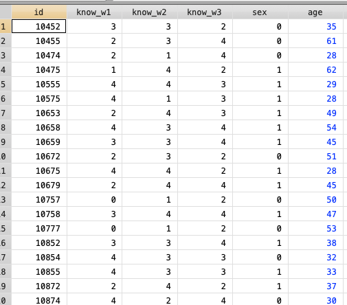
Wide format

The variable “Known” is time variant, that is why we have “known_w1”, “known_w2” and “known_w3”. This variable “known” (political knowledge) has been measured for each individual in three different times. The variable “age” and “sex” for instance, are time “invariant” because haven’t change during this study

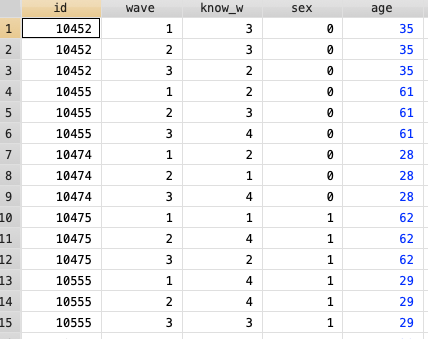
Long format

The structure is different than wide format. The observations repeat for each subject as times were gathered. We can observe that the variable know_w is changing in each “wave” (time) and the variable sex or age does not change for each subject.

1.1.1 STATA

• Lets get the data and keep the variables we need for this example.

use "./datasets/Kenya.3wave wide.2017.dta", clear

keep know_w1 know_w2 know_w3 age sex id age

From wide to long in Stata

reshape long newtreat_ww know_w , i(id) j(wave)

From long to wide in Stata

reshape wide know_w, i(id) j(wave)

1.1.2 R

• First, lets “upload/open” the data set. There are different packages and ways to do it. Here we use the package rio .

• Remember, first install the packages, you can check the list of packages we are using here R packages and data sets.

• You can check other ways here:

  • Upload data to R.
  • Other formats

• After installing the package rio we have to “call” it. For that we use library and it has to be done each session.

• The function import from the package rio recognizes different extensions such as: “.sav”,“xls”,“xlsx”,“DOB”, “csv”, “SAS”, “dta”.. among others. for more info run: ?import

library(rio) ## calling the package
library(dplyr) ## calling the package
data<-import("./datasets/Kenya.3wave wide.2017.dta")

data=data[,c("sex","id","age","know_w1","know_w2","know_w3")]

## Our object "data" has two dimensions: rows, and columns. We can manipulate it using brackets
## [ rows , columns ]
## We keep the columns we need manipulating the second dimension. 

- Different than STATA in R we can have more than one dataset "open". 
- Remeber: R is an object oriented language.
- An object can be a dataset, a map, an image, etc.
- We can have data (with all the variables), 
and data2 with the selected variables "open" at the same time. 
- This is an advantage because we do not need to close our enviroment to change dataset. 
- On a different note, remember: Packages have functions, and functions have arguments!

From wide to long in R

As in STATA this transformation will create a variable wave to point out each time. The values will be: know_w1, know_w2, know_w3.

library(tidyr)
long <- data%>%gather(wave, know_w, -c(id,sex,age))%>%arrange(id) ## Collapse the variables know_w1,know_w2,know_w3 in the new variable know_w
head(long,10)

##    sex    id age    wave know_w
## 1    0 10452  35 know_w1      3
## 2    0 10452  35 know_w2      3
## 3    0 10452  35 know_w3      2
## 4    0 10455  61 know_w1      2
## 5    0 10455  61 know_w2      3
## 6    0 10455  61 know_w3      4
## 7    0 10474  28 know_w1      2
## 8    0 10474  28 know_w2      1
## 9    0 10474  28 know_w3      4
## 10   1 10475  62 know_w1      1

• gather is a tydr function that helps us to reshape the data from wide to long.
• arrange is a dplyr function that sort the data.
• %>% it is a convenient way to concatenate all the steps in one line code.
• head is a base function to show us a glimpse of the data, in this case we asked for the first 10 cases.

From long to wide in R

spreadis a tydr function that it does the oposite of gather

wide <- long%>%spread(wave, know_w)%>%arrange(id) #create the variable know_w for each wave and sort the data by id
head(wide,10) # show some data (10 first rows)

##    sex    id age know_w1 know_w2 know_w3
## 1    0 10452  35       3       3       2
## 2    0 10455  61       2       3       4
## 3    0 10474  28       2       1       4
## 4    1 10475  62       1       4       2
## 5    1 10555  29       4       4       3
## 6    1 10575  28       4       1       3
## 7    1 10653  49       2       4       3
## 8    1 10658  54       4       3       4
## 9    1 10659  45       3       3       4
## 10   0 10672  51       2       3       2

Dplyr and Tidyr are becoming very popular among R users.
That is why we suggest to get use to %>%