In this section, we will use data adapted from:

Civic education, political discussion, and the social transmission of democratic knowledge and values in a new democracy: Kenya 2002. Finkel-Smith (AJPS 2011)

Datasets:

Kenya.3wave wide.2017.dta Download
Kenya.3wave long.2017.dta Download

Effects of US Foreign Assistance on Democracy Building: Results of a Cross-National Quantitative Study (Final report, prepared for USAID) Finkel, Steven E., Anibal Perez-Linan, Mitchell A. Seligson, and Dinorah Azpuru. 2006

Dataset:

democracy.dta Download

Download the files into your computer. We had saved the data-files in a folder called “datasets,” that is why our roots are, for instance: “./datasets/Kenya.3wave wide.2017.dta”

1 Within estimators models

1.1 First Difference two waves

Model:

\[ Y_{it}-Y_{i(t-1)} = X_{1i}-X_{1i(t-1)}+X_{2i}-X_{2i(t-1)}+ \epsilon_i-\epsilon_{i(t-1)}\]

or (Multiwave)

\[ \Delta Y_i= \Delta X_{1i} + \Delta X_{2i} + .. \Delta \epsilon_i\]

Data details

We are going to retrieve the data Finkel-Smith 2011. You can find more details about the data here Datas

This data is in wide format. We will create two variables

Knowdif ($\Delta Knowledge$): difference in knowledge between before and after treatment
newtreat_ww2 ($\Delta Treatment$): binary variable, “1” if the subject got the treatment.

1.1.1 STATA

Creating the variables:

gen knowdif=know_w2-know_w1
gen treatdif=newtreat_ww2-newtreat_ww1
gen intdif=interest_w2-interest_w1

Runing the models

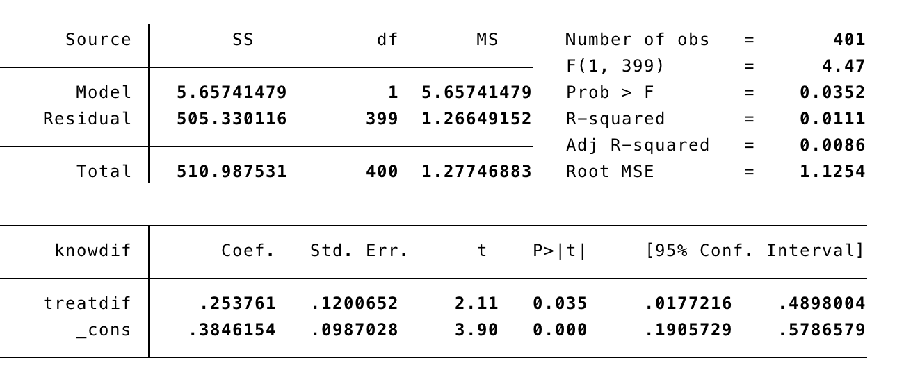
FD_1: First Difference without controls

regress knowdif newtreat_ww2

FD_2: First Difference with controls

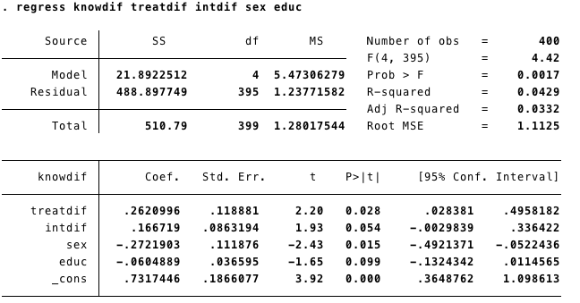
regress knowdif treatdif intdif sex educ

We can add time invariant variables in our model. However the interpretation is not straightforward. For example, in this case, sex and education have negative effects on change in knowledge. This could mean three different things:

- Women increase more on knwoledge than men, and less educated subjects increase more than highly educated. 
- Or: sex and education had greater effects on levels of knowledge at time 1 than time 2.
- Or: sex and education differences were stronger at time 1 than time 2.

1.1.2 R

Now we replicate the models FD_1 and FD_2 using R.

First, we get the data using the function “import” (package rio).
Then we add the variables using “$”.

data=import("./datasets/Kenya.3wave wide.2017.dta")
data$Knowdif=data$know_w2-data$know_w1 ## Variable Knowdif
data$treatdif=data$newtreat_ww2-data$newtreat_ww1 ## Vairable treatdif

Packages as "dplyr" or "tydr" are giving us more options for data management. 
For instance, we can do everything in "one" line of code.
```%>%``` 
(it means: "throw the object/output from the left in to the next function")

In this code below we import the dataset and then “throw” it to the function “mutate” to create new variables (Knowdif and treatdif).
The output is the same.

data=import("./datasets/Kenya.3wave wide.2017.dta")%>%mutate(Knowdif=know_w2-know_w1,treatdif=newtreat_ww2-newtreat_ww1, intdif=interest_w2-interest_w1)

Running the models

First option: Create and object that contains all the information of the model and then ask for the summary of the model.

The function “lm” means “linear model” and it does all the estimation process of the linear model. The dependent and independent variables are separated by “~”, and then, after the coma, we called the data.
The function summary allows us to get relevant information of the model.

FD1=lm(Knowdif~treatdif, data)
summary(FD1)

## 
## Call:
## lm(formula = Knowdif ~ treatdif, data = data)
## 
## Residuals:
##     Min      1Q  Median      3Q     Max 
## -3.6384 -0.6384  0.3616  0.6154  3.6154 
## 
## Coefficients:
##             Estimate Std. Error t value Pr(>|t|)    
## (Intercept)   0.3846     0.0987   3.897 0.000114 ***
## treatdif      0.2538     0.1201   2.114 0.035176 *  
## ---
## Signif. codes:  0 '***' 0.001 '**' 0.01 '*' 0.05 '.' 0.1 ' ' 1
## 
## Residual standard error: 1.125 on 399 degrees of freedom
## Multiple R-squared:  0.01107,    Adjusted R-squared:  0.008593 
## F-statistic: 4.467 on 1 and 399 DF,  p-value: 0.03518

The object “m1” it has more information that was showed in the summary output. For instance, if we want an analysis of variance of the model we can get that with the function “aov”.

aov(FD1)

## Call:
##    aov(formula = FD1)
## 
## Terms:
##                 treatdif Residuals
## Sum of Squares    5.6574  505.3301
## Deg. of Freedom        1       399
## 
## Residual standard error: 1.125385
## Estimated effects may be unbalanced

summary(aov(FD1))

##              Df Sum Sq Mean Sq F value Pr(>F)  
## treatdif      1    5.7   5.657   4.467 0.0352 *
## Residuals   399  505.3   1.266                 
## ---
## Signif. codes:  0 '***' 0.001 '**' 0.01 '*' 0.05 '.' 0.1 ' ' 1

Another option is to run all in one line of code, which could be done using the “%>%”. We throw the linear model into the function summary, in this case we are not saving any object in the memory.

lm(data$Knowdif~data$treatdif, data)%>%summary()

## 
## Call:
## lm(formula = data$Knowdif ~ data$treatdif, data = data)
## 
## Residuals:
##     Min      1Q  Median      3Q     Max 
## -3.6384 -0.6384  0.3616  0.6154  3.6154 
## 
## Coefficients:
##               Estimate Std. Error t value Pr(>|t|)    
## (Intercept)     0.3846     0.0987   3.897 0.000114 ***
## data$treatdif   0.2538     0.1201   2.114 0.035176 *  
## ---
## Signif. codes:  0 '***' 0.001 '**' 0.01 '*' 0.05 '.' 0.1 ' ' 1
## 
## Residual standard error: 1.125 on 399 degrees of freedom
## Multiple R-squared:  0.01107,    Adjusted R-squared:  0.008593 
## F-statistic: 4.467 on 1 and 399 DF,  p-value: 0.03518

Now the model FD2:

We can add more independent/explanatory variables using “+”.

FD2=lm(Knowdif~treatdif+intdif+sex+educ, data)
summary(FD2)

## 
## Call:
## lm(formula = Knowdif ~ treatdif + intdif + sex + educ, data = data)
## 
## Residuals:
##     Min      1Q  Median      3Q     Max 
## -3.5859 -0.6457  0.0209  0.5808  3.3664 
## 
## Coefficients:
##             Estimate Std. Error t value Pr(>|t|)    
## (Intercept)  0.73174    0.18661   3.921 0.000104 ***
## treatdif     0.26210    0.11888   2.205 0.028049 *  
## intdif       0.16672    0.08632   1.931 0.054146 .  
## sex         -0.27219    0.11188  -2.433 0.015419 *  
## educ        -0.06049    0.03660  -1.653 0.099140 .  
## ---
## Signif. codes:  0 '***' 0.001 '**' 0.01 '*' 0.05 '.' 0.1 ' ' 1
## 
## Residual standard error: 1.113 on 395 degrees of freedom
##   (1 observation deleted due to missingness)
## Multiple R-squared:  0.04286,    Adjusted R-squared:  0.03317 
## F-statistic: 4.422 on 4 and 395 DF,  p-value: 0.001655

The interpretation is the same stated above.

1.2 Multiwave First Difference

With the data in long format we can run a Multi Wave First Difference Model:

\[ \Delta Y_i= \Delta X_{1i} + \Delta X_{2i} + .. \Delta \epsilon_i\]

1.2.1 STATA

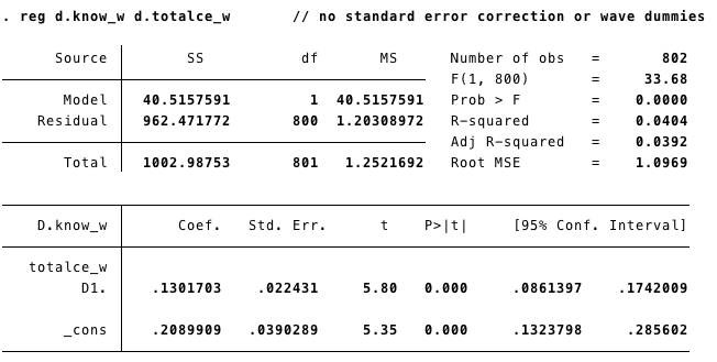
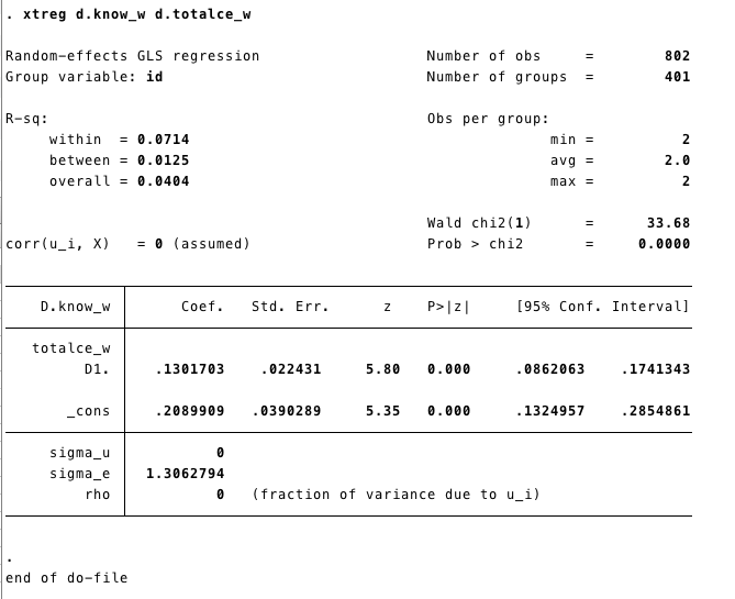
In STATA first we set the data as panel with xtset and then we run the model using d before each variable. This will tell STATA to take the difference of said variable at its previous time and include it in the model.

MWFD1: Multiwave First Difference without waves

xtset id wave
reg d.know_w d.totalce_w

MWFD2: Multiwave First Difference controling by waves(time)

We can run this model controling for the “trend” effect adding the waves.

tab wave, gen(wavv) #//this generates two variables, one for each wave
reg d.know_w d.totalce_w wavv2 wavv3 #// The new model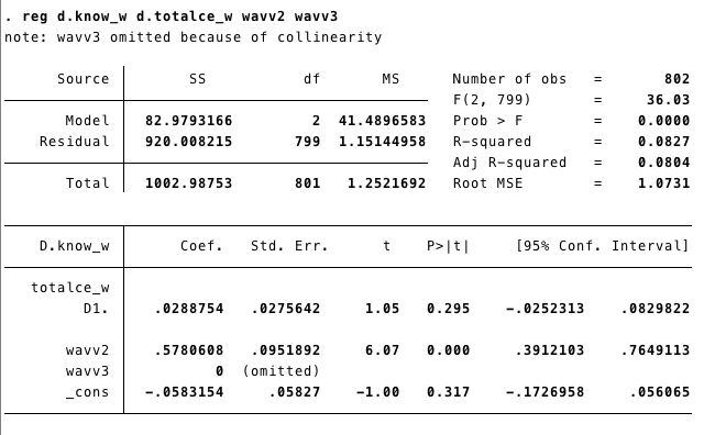

If our data is in a long format, we can also use the xtreg command.

xtset Sets the data as panel.

xtset id wave
xtreg d.know_w d.totalce_w

1.2.2 R

In R we can use the plm package to run a Multiwave First Difference

MWFD1: Multiwave First Difference without waves

First, we call the package plm. Remember we already called the package rio in the step before.
Second, we import the data base using “import”, as we did above.
plm is the function for panel model. As in the linear model, the first element on the function is the model(formula) know_w~totalce_w+age+educ+sex.
Variables are added using +. Then we include the data data =K_long. - The third element in our code is the “index” index = c("id", "wave"), which does the same job that “xtset” in STATA.
Finally, we need to specified the type of model model = "fd". We have several options here that we will be unveiling as we progress.
summary(MWFD1) shows us the results.

library(plm)

K_long<-import("./datasets/Kenya.3wave long.2017.dta")  ### Here I'm importing the data.

MWFD1<-plm(know_w~totalce_w+age+educ+sex,data =K_long,
          index = c("id", "wave"), 
          model = "fd")
summary(MWFD1)

## Oneway (individual) effect First-Difference Model
## 
## Call:
## plm(formula = know_w ~ totalce_w + age + educ + sex, data = K_long, 
##     model = "fd", index = c("id", "wave"))
## 
## Balanced Panel: n = 401, T = 3, N = 1203
## Observations used in estimation: 802
## 
## Residuals:
##      Min.   1st Qu.    Median   3rd Qu.      Max. 
## -3.469332 -0.599502 -0.078821  0.791009  3.791009 
## 
## Coefficients:
##             Estimate Std. Error t-value  Pr(>|t|)    
## (Intercept) 0.208991   0.039029  5.3548 1.120e-07 ***
## totalce_w   0.130170   0.022431  5.8031 9.377e-09 ***
## ---
## Signif. codes:  0 '***' 0.001 '**' 0.01 '*' 0.05 '.' 0.1 ' ' 1
## 
## Total Sum of Squares:    1003
## Residual Sum of Squares: 962.47
## R-Squared:      0.040395
## Adj. R-Squared: 0.039196
## F-statistic: 33.6764 on 1 and 800 DF, p-value: 9.3768e-09

MWFD2: Multiwave First Difference controling by waves(time)

First, we need to create a dummy for each wave. There are different ways to create dummy variables. We are going to use the function mutate from dplyr. We have used that function here

K_long<-K_long%>%mutate(wavv1=ifelse(wave==1,1,0),
                        wavv2=ifelse(wave==2,1,0),
                        wavv3=ifelse(wave==3,1,0))

Now we can include waves in the model. Two waves are omited due to multicoliniarity.

FDMW2<-plm(know_w~totalce_w+wavv1+wavv2,data =K_long,
          index = c("id", "wave"), 
          model = "fd")
summary(FDMW2)

## Oneway (individual) effect First-Difference Model
## 
## Call:
## plm(formula = know_w ~ totalce_w + wavv1 + wavv2, data = K_long, 
##     model = "fd", index = c("id", "wave"))
## 
## Balanced Panel: n = 401, T = 3, N = 1203
## Observations used in estimation: 802
## 
## Residuals:
##      Min.   1st Qu.    Median   3rd Qu.      Max. 
## -3.577496 -0.606372  0.087191  0.480255  3.480255 
## 
## Coefficients: (1 dropped because of singularities)
##              Estimate Std. Error t-value  Pr(>|t|)    
## (Intercept) -0.058315   0.058270 -1.0008    0.3172    
## totalce_w    0.028875   0.027564  1.0476    0.2952    
## wavv1       -0.578061   0.095189 -6.0728 1.943e-09 ***
## ---
## Signif. codes:  0 '***' 0.001 '**' 0.01 '*' 0.05 '.' 0.1 ' ' 1
## 
## Total Sum of Squares:    1003
## Residual Sum of Squares: 920.01
## R-Squared:      0.082732
## Adj. R-Squared: 0.080436
## F-statistic: 36.0325 on 2 and 799 DF, p-value: 1.0404e-15

1.3 Simple FE

Two more common models:

\[Y_{it}=\alpha + \beta_1X_{1it}+...\beta_kX_{ikt}+\beta_mZ_i+c_1D_1+c_2D_2+c_{n-1}D_{n-1}+e_{it}\]

In the model above we add a dummy variable (“D”) for each unit; this model is common called (“Least Squares Dummy Variables”). Then each unite will have its own intercept. For instance ($\alpha +c1$) for unite 1. A drawback with this model is that it is too computationally demanding, especially if we have a large number of units.

The most common model is the Fixed Effect model:

\[Y_{it}-\bar{Y_i}=\beta_i(X_{1it}-\bar{X}_{1i})+...+ \beta_k(X_{kit}-\bar{X}_{ki})+ \epsilon_{it}\]

These models control for the variation between units and only use the within estimators.

To estimate these models we are going to use the data from Finkel-Smith 2011 in its long format. You can download it from here: Datas

1.3.1 STATA

xtset sets the data as panel. gen creates or generates a new variable “time” (starts in 0)

xtset id wave
gen time=wave-1

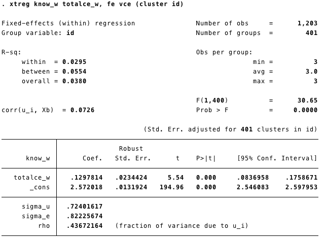
Runing the model

Know_w = level of knowledge.
tatalce_w=
fe means fixed effect

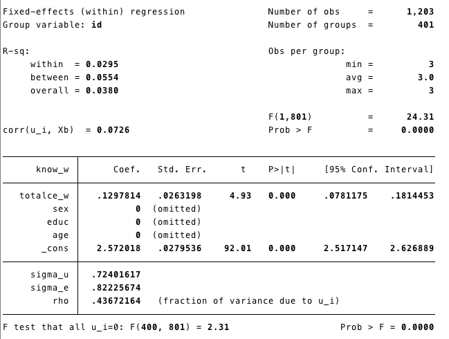
xtreg know_w totalce_w sex educ age, fe

Time invariants covariates were eliminated from the model (because they do not vary within subjects!)

1.3.2 R

There are several packages that can help us to estimate panel models. There is some overlapping, as some packages can take a specific approach for a given problem. For instance plm was created by econometricians and panelR by a sociologist. The best practice is to use the package that can help us with our analysis and not to get attached to any in particular.
Here is a good post from panelR’s author comparing his package with plm. Post

R- plm

If you hadn’t uploaded the dataset before remember:
First, we call the package.
Second, we import the database using “import”
plm is the function for panel model. As the linear model, the first element is the model know_w~totalce_w+age+educ+sex. Variables are added using +. then we include the data data =K_long. The third element in our code is the “index” index = c("id", "wave") which does the same job that “xtset” in STATA. Finally, we need to specify the type of model model = "within". We have several options here, that we are unveiling as we progress.
summary(FE) shows us the results.

We do not have to call the package everytime we run a function, only once in a session. 

For instance we called library(rio) before, therefore we do not need to call it again

K_long<-import("./datasets/Kenya.3wave long.2017.dta")
FE<-plm(know_w~totalce_w+age+educ+sex,data =K_long,
        index = c("id", "wave"), 
        model = "within")
summary(FE)

## Oneway (individual) effect Within Model
## 
## Call:
## plm(formula = know_w ~ totalce_w + age + educ + sex, data = K_long, 
##     model = "within", index = c("id", "wave"))
## 
## Balanced Panel: n = 401, T = 3, N = 1203
## 
## Residuals:
##     Min.  1st Qu.   Median  3rd Qu.     Max. 
## -2.53689 -0.37022  0.00000  0.41348  2.08652 
## 
## Coefficients:
##           Estimate Std. Error t-value  Pr(>|t|)    
## totalce_w  0.12978    0.02632  4.9309 9.951e-07 ***
## ---
## Signif. codes:  0 '***' 0.001 '**' 0.01 '*' 0.05 '.' 0.1 ' ' 1
## 
## Total Sum of Squares:    558
## Residual Sum of Squares: 541.56
## R-Squared:      0.029461
## Adj. R-Squared: -0.45642
## F-statistic: 24.3142 on 1 and 801 DF, p-value: 9.9511e-07

The summary of the model does not give us the “intercept”. STATA estimates the intercept running the model after adding the overall sample mean for Y and X to the demeaned X and Y.

plm has a function to obtain it

within_intercept(FE)

## (overall_intercept) 
##            2.572018 
## attr(,"se")
## [1] 0.0279536

In this case the result is the same as the output from the STATA command.

R- panelR

First, we call the package ‘panelR’ before using it.
We “panel” our data panel_data(K_long, id=id, wave=wave). We created a new object (K_long_p). We could also replace the previous one.

library(panelr) 
K_long_p<-panel_data(K_long, id=id, wave=wave)
head(K_long_p)

## # Panel data:    6 x 17
## # entities:      id [2]
## # wave variable: wave [1, 2, 3 (3 waves)]
##   id     wave wave1 treat newtreat_ww evertreat totalce_w talknum_w
##   <fct> <dbl> <dbl> <dbl>       <dbl>     <dbl>     <dbl>     <dbl>
## 1 10452     1     0     1           0         1         0         0
## 2 10452     2     1     1           1         1         1         1
## 3 10452     3     2     1           0         1         0         0
## 4 10455     1     0     1           0         1         0         0
## 5 10455     2     1     1           1         1         1         3
## 6 10455     3     2     1           0         1         0         0
## # … with 9 more variables: interest_w <dbl>, media_w <dbl>, know_w <dbl>,
## #   polpart_w <dbl>, polprt2_w <dbl>, sex <dbl>, age <dbl>, educ <dbl>,
## #   totalce_mn <dbl>

Second, we run the model using the function “wbm”. The structure is the same as “plm”.

FE2<-wbm(know_w~totalce_w+age+educ+sex, data=K_long_p,
        model="within")

## Warning: Constants are ignored with within model specifications.

summary(FE2)

## MODEL INFO:
## Entities: 401
## Time periods: 1-3
## Dependent variable: know_w
## Model type: Linear mixed effects
## Specification: within
## 
## MODEL FIT:
## AIC = 3314.29, BIC = 3334.66
## Pseudo-R² (fixed effects) = 0.01
## Pseudo-R² (total) = 0.33
## Entity ICC = 0.32
## 
## --------------------------------------------------------
##                     Est.   S.E.   t val.     d.f.      p
## ----------------- ------ ------ -------- -------- ------
## (Intercept)         2.65   0.04    71.67   400.00   0.00
## totalce_w           0.13   0.03     4.93   801.00   0.00
## --------------------------------------------------------
## 
## p values calculated using Satterthwaite d.f.
##  
## RANDOM EFFECTS:
## ------------------------------------
##   Group      Parameter    Std. Dev. 
## ---------- ------------- -----------
##     id      (Intercept)    0.5664   
##  Residual                  0.8223   
## ------------------------------------

1.4 Two ways FE

We can control for time, adding time dummies to our FE model. This is common called two ways (time-and-cluster) fixed effect.

1.4.1 STATA

We use the same components of our previous fixed effect model (fe).

We create new variables for each wave.

tab wave, gen(wavv)

We include the time dummies to our fe model!

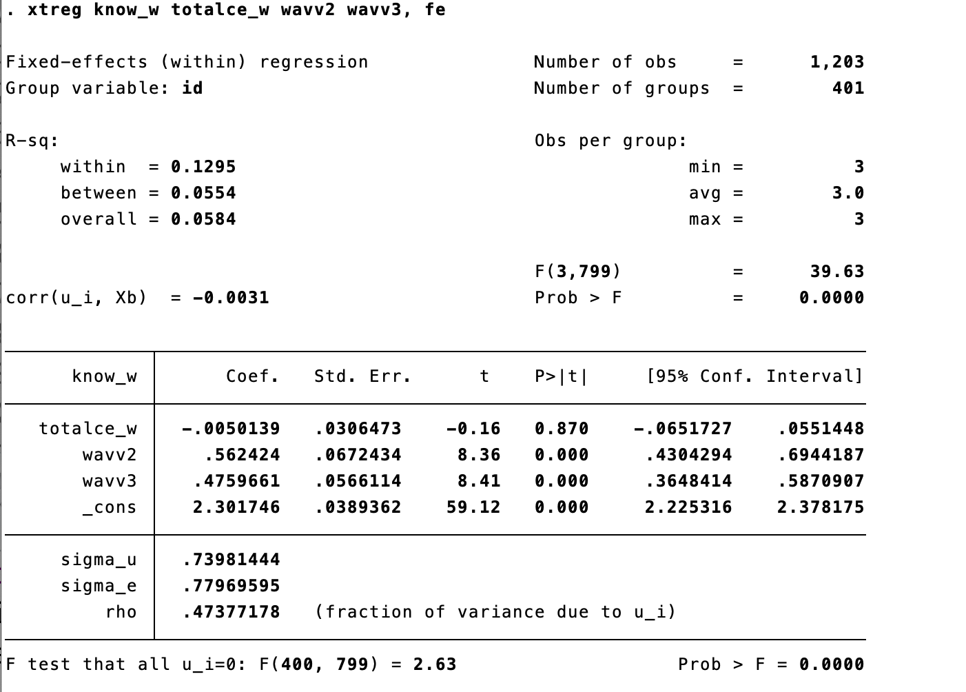
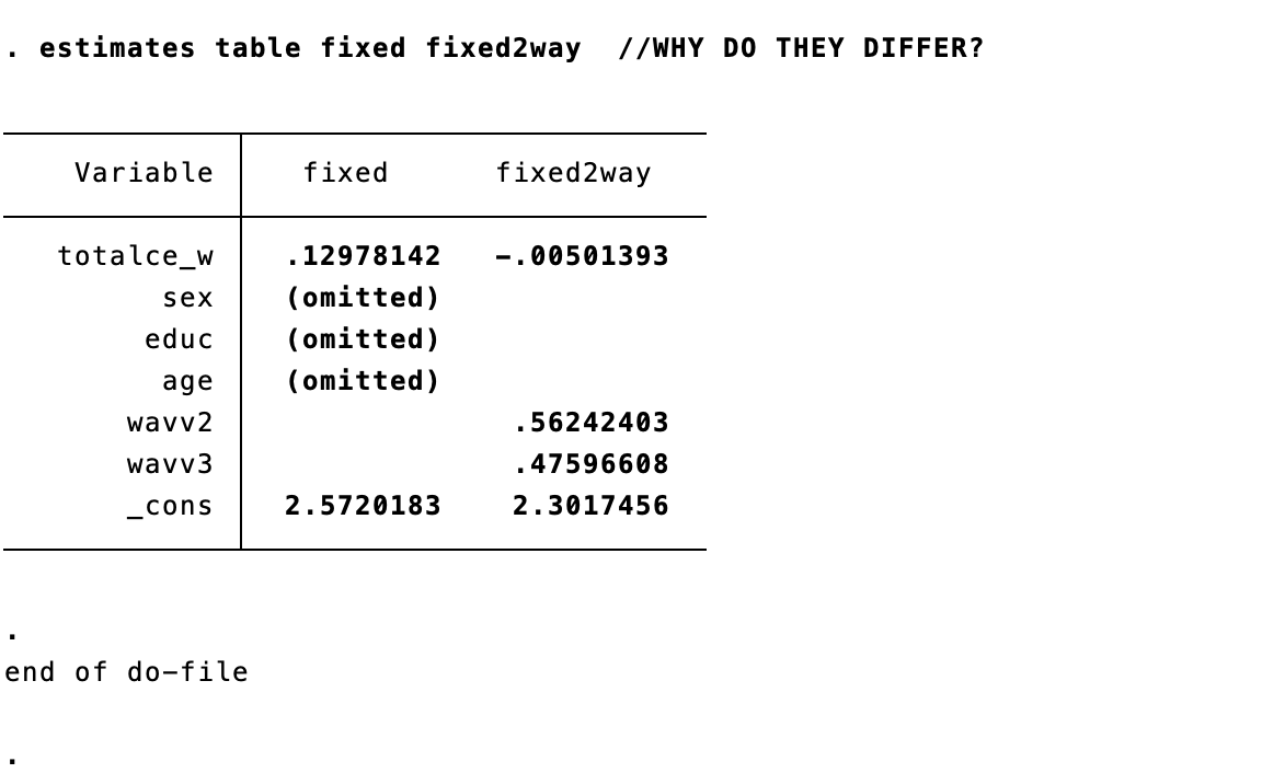
xtreg know_w totalce_w wavv2 wavv3, fe

The results of our main variable had changed!- We can compare the estimates. The effect main variable have changed, therefore in this case it was important to include the time effect.

1.4.2 R

We can replicate this with R using the “plm” package. as.factor(wave) plays the same role with tab wave, gen(wavv) in Stata.

fixed2way<- plm(data=K_long, know_w ~ totalce_w+as.factor(wave))

summary(fixed2way)

## Oneway (individual) effect Within Model
## 
## Call:
## plm(formula = know_w ~ totalce_w + as.factor(wave), data = K_long)
## 
## Balanced Panel: n = 401, T = 3, N = 1203
## 
## Residuals:
##       Min.    1st Qu.     Median    3rd Qu.       Max. 
## -2.3255506 -0.4631694  0.0077828  0.4537153  2.3461300 
## 
## Coefficients:
##                    Estimate Std. Error t-value  Pr(>|t|)    
## totalce_w        -0.0050139  0.0306473 -0.1636    0.8701    
## as.factor(wave)2  0.5624240  0.0672434  8.3640 2.688e-16 ***
## as.factor(wave)3  0.4759661  0.0566114  8.4076 < 2.2e-16 ***
## ---
## Signif. codes:  0 '***' 0.001 '**' 0.01 '*' 0.05 '.' 0.1 ' ' 1
## 
## Total Sum of Squares:    558
## Residual Sum of Squares: 485.73
## R-Squared:      0.12951
## Adj. R-Squared: -0.30955
## F-statistic: 39.6251 on 3 and 799 DF, p-value: < 2.22e-16

As we mentioned before STATA show the intercept as part of the results of FE models, and R doesn’t. However, we can obtained it using the plm package.

within_intercept(fixed2way)

## (overall_intercept) 
##            2.301746 
## attr(,"se")
## [1] 0.03893616

1.5 FE, robust standard errors (RSE).

We can deal with the heteroskedasticity of the error terms obtaining the “ROBUST” standard errors. Panel analysis has potential problems with the error terms produced by unit-level clustering.

1.5.1 STATA

xtreg know_w totalce_w, fe (cluster id)

As we can see, now the SE are “robust”.

1.5.2 R

R- plm

We have more than one option to get the robust standard errors from our model.
With PLM we can add the argument vcov in summary()
Remember: our model was stored in the object FE above.

summary(FE,vcov = vcovHC(FE))

## Oneway (individual) effect Within Model
## 
## Note: Coefficient variance-covariance matrix supplied: vcovHC(FE)
## 
## Call:
## plm(formula = know_w ~ totalce_w + age + educ + sex, data = K_long, 
##     model = "within", index = c("id", "wave"))
## 
## Balanced Panel: n = 401, T = 3, N = 1203
## 
## Residuals:
##     Min.  1st Qu.   Median  3rd Qu.     Max. 
## -2.53689 -0.37022  0.00000  0.41348  2.08652 
## 
## Coefficients:
##           Estimate Std. Error t-value  Pr(>|t|)    
## totalce_w 0.129781   0.023403  5.5454 3.984e-08 ***
## ---
## Signif. codes:  0 '***' 0.001 '**' 0.01 '*' 0.05 '.' 0.1 ' ' 1
## 
## Total Sum of Squares:    558
## Residual Sum of Squares: 541.56
## R-Squared:      0.029461
## Adj. R-Squared: -0.45642
## F-statistic: 30.7516 on 1 and 400 DF, p-value: 5.3379e-08

Another option is to use a generic function to test our coeficients. The function coeftest from the package lmtest performs z and t Wald tests (significance) of the estimated coefficients.
The argument vcov allows us to select a particular variance-covariance matrix.

library(lmtest)
coeftest(FE, vcov = vcovHC, type = "HC1")

## 
## t test of coefficients:
## 
##           Estimate Std. Error t value  Pr(>|t|)    
## totalce_w 0.129781   0.023413  5.5431 4.035e-08 ***
## ---
## Signif. codes:  0 '***' 0.001 '**' 0.01 '*' 0.05 '.' 0.1 ' ' 1

Now we get the robust standard error for the intercept.

within_intercept(FE, vcov = function(x) 
  vcovHC(x, type="HC1"))

## (overall_intercept) 
##            2.572018 
## attr(,"se")
## [1] 0.01318144

R- panelR

Panel R has not yet implemented yet a easy way to test the coefficients with Robust Standard Error.

1.6 Random Effects Models

Also known as Random Intercept

1.6.1 STATA

We also use xtreg for random effects model.
We add theta ($\theta$) in the line. Because $\theta$ gives us an idea of the error term’s compositions. As $\theta$ (theta) gets closer to 1, it means that more and more of the composite error variance is made up of $U_i$ unit-level or “between” variance. Where $\theta$ closser to 1 the RE models reduce to a FE model

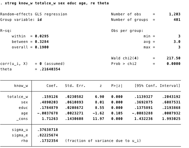
xtreg know_w totalce_w sex educ age, re theta

We can also add Robust Standard Errors to the model. We added vce(cluster id) same as we did with the Fixed Effects model.

xtreg know_w totalce_w sex educ age, re vce (cluster id)

1.6.2 R

We run the model using the function plm from the package with the same name.
The code follows the same structure as the FE or Multiwave First Difference showed above.
The difference is in model we select random: model = "random"

RE<-plm(know_w~totalce_w+age+educ+sex,data =K_long,
        index = c("id", "wave"), 
        model = "random")

summary(RE)

## Oneway (individual) effect Random Effect Model 
##    (Swamy-Arora's transformation)
## 
## Call:
## plm(formula = know_w ~ totalce_w + age + educ + sex, data = K_long, 
##     model = "random", index = c("id", "wave"))
## 
## Balanced Panel: n = 401, T = 3, N = 1203
## 
## Effects:
##                  var std.dev share
## idiosyncratic 0.6761  0.8223 0.827
## individual    0.1417  0.3764 0.173
## theta: 0.2164
## 
## Residuals:
##       Min.    1st Qu.     Median    3rd Qu.       Max. 
## -2.5409793 -0.5741804 -0.0045051  0.6213067  2.1813203 
## 
## Coefficients:
##               Estimate Std. Error z-value  Pr(>|z|)    
## (Intercept)  1.7126305  0.1430608 11.9713 < 2.2e-16 ***
## totalce_w    0.1591260  0.0230582  6.9011 5.162e-12 ***
## age         -0.0037678  0.0023271 -1.6191    0.1054    
## educ         0.1784879  0.0208672  8.5535 < 2.2e-16 ***
## sex          0.4890203  0.0610893  8.0050 1.195e-15 ***
## ---
## Signif. codes:  0 '***' 0.001 '**' 0.01 '*' 0.05 '.' 0.1 ' ' 1
## 
## Total Sum of Squares:    960.45
## Residual Sum of Squares: 812.87
## R-Squared:      0.15366
## Adj. R-Squared: 0.15083
## Chisq: 217.505 on 4 DF, p-value: < 2.22e-16

summary(RE) give us the basic information from the model.
The results are the same as the STATA output, and plm give us $\theta$ by default.

Robust standard errors

We can get the **robust standard errors adding the argument in the function summary() as we did with FE models

summary(RE, vcov = vcovHC(RE))

## Oneway (individual) effect Random Effect Model 
##    (Swamy-Arora's transformation)
## 
## Note: Coefficient variance-covariance matrix supplied: vcovHC(RE)
## 
## Call:
## plm(formula = know_w ~ totalce_w + age + educ + sex, data = K_long, 
##     model = "random", index = c("id", "wave"))
## 
## Balanced Panel: n = 401, T = 3, N = 1203
## 
## Effects:
##                  var std.dev share
## idiosyncratic 0.6761  0.8223 0.827
## individual    0.1417  0.3764 0.173
## theta: 0.2164
## 
## Residuals:
##       Min.    1st Qu.     Median    3rd Qu.       Max. 
## -2.5409793 -0.5741804 -0.0045051  0.6213067  2.1813203 
## 
## Coefficients:
##               Estimate Std. Error z-value  Pr(>|z|)    
## (Intercept)  1.7126305  0.1593532 10.7474 < 2.2e-16 ***
## totalce_w    0.1591260  0.0206163  7.7184 1.178e-14 ***
## age         -0.0037678  0.0027063 -1.3922    0.1639    
## educ         0.1784879  0.0241090  7.4034 1.328e-13 ***
## sex          0.4890203  0.0632721  7.7288 1.085e-14 ***
## ---
## Signif. codes:  0 '***' 0.001 '**' 0.01 '*' 0.05 '.' 0.1 ' ' 1
## 
## Total Sum of Squares:    960.45
## Residual Sum of Squares: 812.87
## R-Squared:      0.15366
## Adj. R-Squared: 0.15083
## Chisq: 260.397 on 4 DF, p-value: < 2.22e-16

1.7 Hausman test

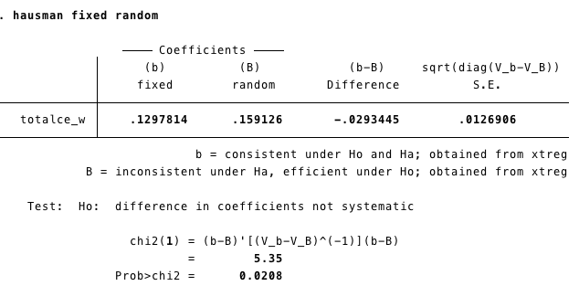
If you are unsure about if to use FE or RE, the Hausman Test (HT) can help you to decide. The HT tests if the estimates obtained by the Fixed Effect models are the same as those from the Random Effect model. If they are the same, RE it is more efficient.

The test statistic is :

\[ \frac{\beta_{Fe}-\beta_{RE}}{var(\beta_{FE})-var(\beta_{RE})} \]

With a $\chi^2$ (Chi-square) with degree of freedom equal to the number of time-varying independent variables.

1.7.1 STATA

To conduct the Hausman Test we need to store the coefficient from our Fixed Effect and Random Effects model.

qui is to estimate the model but no showing the output.
estimate store save the estimates from the model in the “object” fixed and random respectively.

qui xtreg know_w totalce_w sex educ age, fe  
estimates store fixed

qui xtreg know_w totalce_w sex educ age, re theta
estimates store random

We conduct the Hausman test using the command: hausman fixed random

hausman fixed random

1.7.2 R

The package plm has a function called phtest to conduct the Hausman test.

We have created the models before, but we will do it again to be sure we are comparing the right estimators.

FE<-plm(know_w~totalce_w+age+educ+sex,data =K_long,
        index = c("id", "wave"), 
        model = "within") 

RE<-plm(know_w~totalce_w+age+educ+sex,data =K_long,
        index = c("id", "wave"), 
        model = "random")

Now we can conduct the Hausman test.

phtest(FE, RE)

## 
##  Hausman Test
## 
## data:  know_w ~ totalce_w + age + educ + sex
## chisq = 5.3468, df = 1, p-value = 0.02076
## alternative hypothesis: one model is inconsistent

Another way: phtest let us run the test withour re-running the model
We create the object model that contains the name of the dependent and independent variables (separated by ~)

modht= know_w~totalce_w+age+educ+sex #an object with the model 
phtest(modht, data=K_long)  #We can run the test with the model.

## 
##  Hausman Test
## 
## data:  modht
## chisq = 5.3468, df = 1, p-value = 0.02076
## alternative hypothesis: one model is inconsistent

2 Hybrid Models

2.1 Bell and Jones Model with RSE

It includes the mean of the time variant variables into an RE model
First we generate the mean of totalce_w by group and then include it in the model.

2.1.1 STATA

egen totalce_mn=mean(totalce_w), by (id) // egen creates new  variables

xtreg polpart_w totalce_w totalce_mn sex educ age wavv2 wavv3, re vce(cluster id)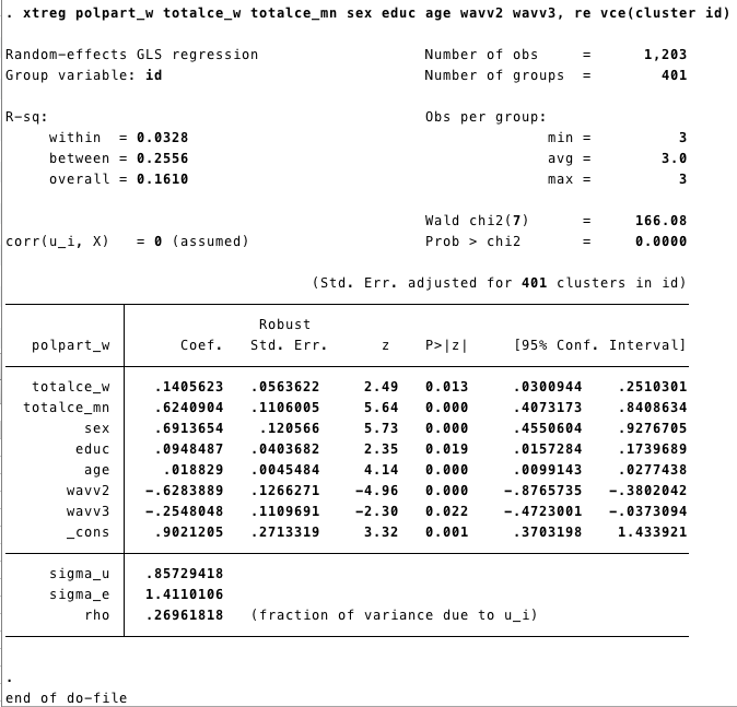

2.1.2 R

First, we create totalce_mn, which is the mean of totalce_w by group. To do this, we will use the function mutate from the package dplyr.
We are going to use the dummys variables for wave. We had created those dummies using mutate for the Multiwave First Difference model here
We can do it again, just in case:

K_long<-K_long%>%mutate(wavv1=ifelse(wave==1,1,0),
                        wavv2=ifelse(wave==2,1,0),
                        wavv3=ifelse(wave==3,1,0))

K_long<-K_long%>%group_by(id)%>%
  mutate(totalce_mn=mean(totalce_w))%>%
  ungroup() # if you don't ungroup you may encounter the following error: 
#Can't join on '.rows' x '.rows' because of incompatible types (list / list)

We include the mean of totalce_w by group in our Random Effects model. Using plm we obtained the same results as STATA
In summary we added the vcov option to request the robust standard errors.

HY<-plm(polpart_w~totalce_w+totalce_mn+age+educ+sex+
           wavv2+wavv3,data =K_long,
         index = c("id", "wave"), 
         model = "random") ## 

summary(HY, vcov = vcovHC(HY))

## Oneway (individual) effect Random Effect Model 
##    (Swamy-Arora's transformation)
## 
## Note: Coefficient variance-covariance matrix supplied: vcovHC(HY)
## 
## Call:
## plm(formula = polpart_w ~ totalce_w + totalce_mn + age + educ + 
##     sex + wavv2 + wavv3, data = K_long, model = "random", index = c("id", 
##     "wave"))
## 
## Balanced Panel: n = 401, T = 3, N = 1203
## 
## Effects:
##                  var std.dev share
## idiosyncratic 1.9910  1.4110  0.73
## individual    0.7350  0.8573  0.27
## theta: 0.3112
## 
## Residuals:
##     Min.  1st Qu.   Median  3rd Qu.     Max. 
## -3.68686 -1.01358 -0.16687  0.93524  4.30400 
## 
## Coefficients:
##               Estimate Std. Error z-value  Pr(>|z|)    
## (Intercept)  0.9021205  0.2702031  3.3387 0.0008418 ***
## totalce_w    0.1405623  0.0561277  2.5043 0.0122684 *  
## totalce_mn   0.6240904  0.1101404  5.6663 1.459e-08 ***
## age          0.0188290  0.0045295  4.1570 3.225e-05 ***
## educ         0.0948487  0.0402003  2.3594 0.0183043 *  
## sex          0.6913654  0.1200645  5.7583 8.497e-09 ***
## wavv2       -0.6283889  0.1261004 -4.9832 6.253e-07 ***
## wavv3       -0.2548048  0.1105074 -2.3058 0.0211235 *  
## ---
## Signif. codes:  0 '***' 0.001 '**' 0.01 '*' 0.05 '.' 0.1 ' ' 1
## 
## Total Sum of Squares:    2703.8
## Residual Sum of Squares: 2379.2
## R-Squared:      0.12004
## Adj. R-Squared: 0.11489
## Chisq: 167.474 on 7 DF, p-value: < 2.22e-16

Hybrid model using panelR package

panelr has a convenient way to estimate an hybrid model.

First we need to panel the data:

K_longp<-panel_data(K_long, id = id, wave = wave)

The structure of the model is the following:

dv ~ varying_variables | invariant_variables | cross_level_interactions/random effects

our varying variables are : totalce_w , and wavv2 + wavv3
Time invariant variables: age, educ, sex
Random effect: id

model <- wbm(polpart_w ~totalce_w + wavv2+wavv3| totalce_w + age + educ + sex | id, data = K_longp)

## fixed-effect model matrix is rank deficient so dropping 2 columns / coefficients

summary(model)

## MODEL INFO:
## Entities: 401
## Time periods: 1-3
## Dependent variable: polpart_w
## Model type: Linear mixed effects
## Specification: within-between
## 
## MODEL FIT:
## AIC = 4585.88, BIC = 4636.8
## Pseudo-R² (fixed effects) = 0.16
## Pseudo-R² (total) = 0.39
## Entity ICC = 0.27
## 
## WITHIN EFFECTS:
## -------------------------------------------------------
##                    Est.   S.E.   t val.     d.f.      p
## --------------- ------- ------ -------- -------- ------
## totalce_w          0.14   0.06     2.53   799.00   0.01
## wavv2             -0.63   0.12    -5.16   799.00   0.00
## wavv3             -0.25   0.10    -2.49   799.00   0.01
## -------------------------------------------------------
## 
## BETWEEN EFFECTS:
## -------------------------------------------------------------
##                          Est.   S.E.   t val.     d.f.      p
## ---------------------- ------ ------ -------- -------- ------
## (Intercept)              0.61   0.28     2.16   396.00   0.03
## imean(totalce_w)         0.76   0.09     8.25   396.00   0.00
## age                      0.02   0.00     4.15   396.00   0.00
## educ                     0.09   0.04     2.33   396.00   0.02
## sex                      0.69   0.12     5.80   396.00   0.00
## -------------------------------------------------------------
## 
## p values calculated using Satterthwaite d.f.
##  
## RANDOM EFFECTS:
## ------------------------------------
##   Group      Parameter    Std. Dev. 
## ---------- ------------- -----------
##     id      (Intercept)    0.8573   
##  Residual                   1.411   
## ------------------------------------

3 Dynamic Models

Panel econometric models can include dynamic effects. There are different kinds of dynamic models those can include lag dependent variable, lag independent

\[ Y_{it}= \alpha+ \beta_1Y_{it-1}+\beta_2X_{it}+\beta_3X_{it-1}+...U_{it}+\epsilon_{it} \]

The problem to include the lag dependent variable is that the estimator would be biased because the lag dependent variable is correlated with $U$ (the time invariant unobserved component of the error term)

The most well know approach is the proposeb by Arellano and Bond that use the lag variables as instruments.

3.0.1 STATA

We are going to use the data “democracy.dta”. More details about the data here: Data
First, we set the data as panel data with xtset
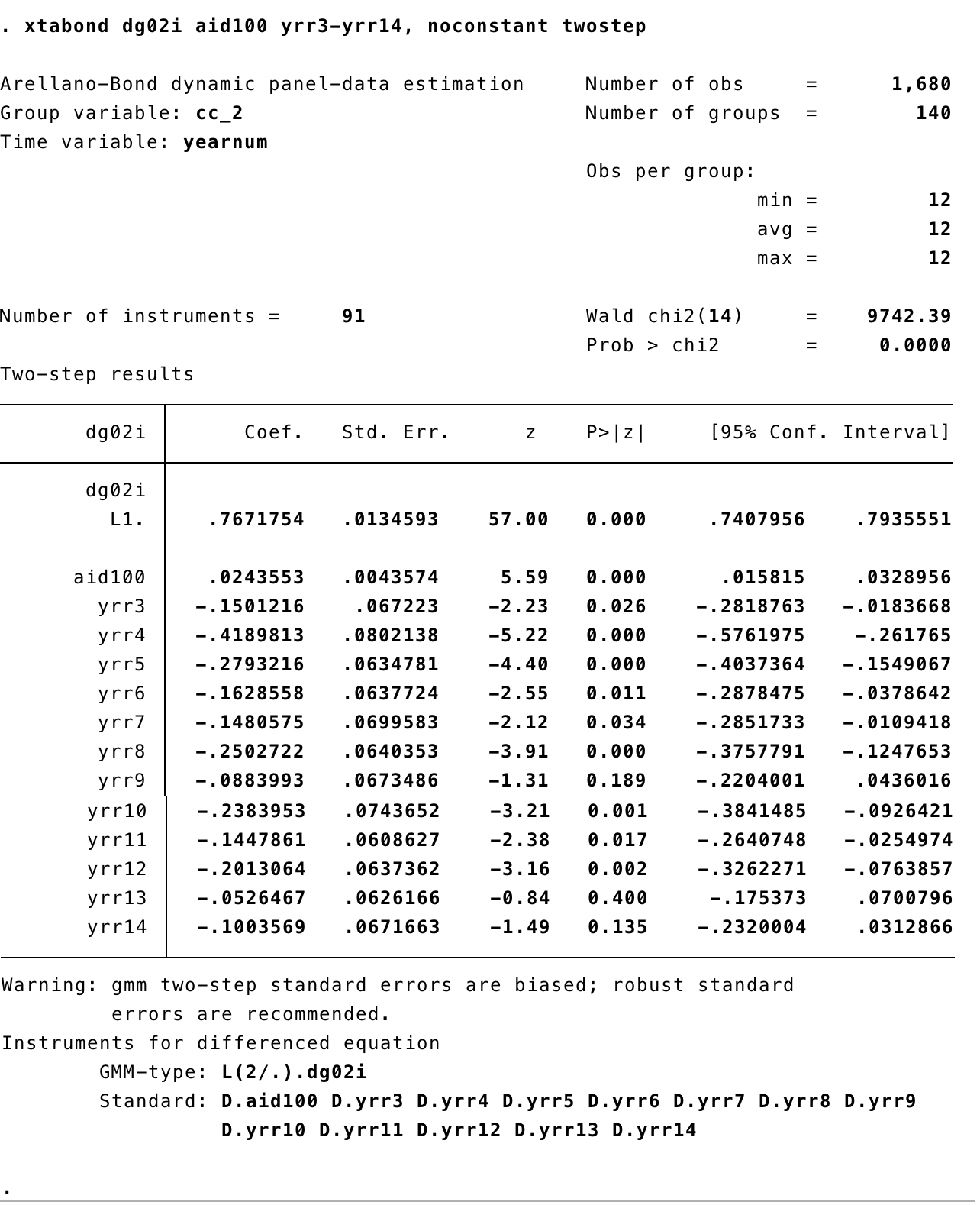
Second, we are going to creat a dummy variable for each year to use them as control variables using the command tab
Finally, we use the command xtabond to estimate the Arellano Bond (1991) model also known as “Generalized Method of Moments (GMM)”

xtset cc_2 yearnum
tab yearnum, gen(yrr)

use "./datasets/democracy.dta"

xtabond dg02i aid100 yrr3-yrr14, noconstant twostep

Output

3.0.2 R

For GMM models we can use the function pgmm from the package plm.
First, lets get the data with the function import from the package rio

demo<-import("./datasets/democracy.dta")

Now the model. The basic model follows the same estructure of the lineal models we ran before: ~ separates the dependent and independent variables
In this model we have aid100 and the lag of dg02i as independent variables.
The other lags (from t-3 to t-14) are used as instruments. We add those using |lag(dg02i,2:14)
We index index=c("cname","year") to let R know the structure of our data.
We run the model in two steps, this is the same as STATA.

dynamic1<-pgmm(dg02i~ aid100+lag(dg02i,1)| lag(dg02i,2:14), data = demo,
         index=c("cname","year"),
         effect = "twoways", model = "twosteps")